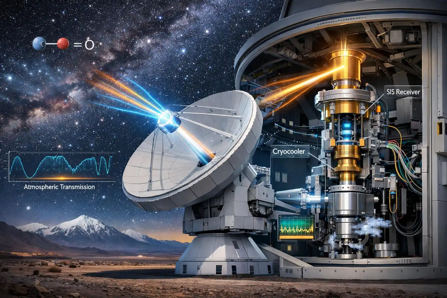

When astronomers talk about ALMA—the Atacama Large Millimeter/submillimeter Array—they often focus on the science: protoplanetary disks, high-redshift galaxies, molecular clouds. What gets less attention is the receiver cartridge sitting at the Cassegrain focus of each of those sixty-six antennas, the device that actually converts faint submillimeter photons into measurable voltages. Today I want to walk through one specific piece of that chain: Band 6, ALMA’s workhorse receiver covering 211 to 275 GHz, and explain why this particular frequency window matters, how the instrument achieves its sensitivity, and what limits its performance on the Chajnantor Plateau.
Why 211–275 GHz?
Band 6 sits squarely in the atmospheric window between two water-vapor absorption features. At ALMA’s 5000-meter altitude, precipitable water vapor (PWV)—the integrated column of water above the site—averages around 1 mm during good observing conditions, dropping below 0.5 mm on the best nights. Water absorbs strongly near 183 GHz and again above 325 GHz, but the Band 6 range enjoys relatively low opacity: typical zenith optical depths run 0.03 to 0.10 at 230 GHz when PWV is 1 mm. That translates to atmospheric transmission of 97% to 90% straight overhead, degrading as you observe lower elevations where the slant path through the atmosphere lengthens.
This frequency range captures the J = 2→1 rotational transition of carbon monoxide (¹²CO) at 230.538 GHz, one of the most-used tracers of molecular gas in the universe. Redshift that line by z = 0.2 and it lands at 192 GHz (Band 5 territory); push to z = 2 and you’re at 77 GHz (Band 3). But for nearby galaxies, protoplanetary disks in Taurus or Ophiuchus, and star-forming regions within a few kiloparsecs, Band 6 delivers CO(2–1) along with dozens of other molecular lines: CS(5–4) at 244.9 GHz, ¹³CO(2–1) at 220.4 GHz, C¹⁸O(2–1) at 219.6 GHz, and the spectral forest of complex organics like CH₃OH and CH₃CN that light up in hot cores.
The band also covers continuum emission from cold dust. A 20-Kelvin dust grain radiating as a blackbody peaks in B_ν near 1 THz, and a modified blackbody peaks at still higher frequency, but 230 GHz remains on the low-frequency side of the spectrum where the flux density scales predictably with dust mass if you know the temperature and opacity law. Band 6 continuum maps reveal the mass reservoirs feeding star formation, the dust disks around young stars, and the thermal emission from distant galaxies whose starlight has heated interstellar grains.
Superconductor-Insulator-Superconductor Mixers
The receiver cartridge itself is a cryogenic heterodyne system. Incoming sky signal enters through a corrugated feedhorn, passes through an orthomode transducer (OMT) that splits the radiation into two orthogonal linear polarizations, and each polarization channel feeds a superconductor-insulator-superconductor (SIS) mixer. The SIS junction is a thin tunnel barrier—niobium-aluminum oxide-niobium, a few nanometers thick—that exhibits a sharp nonlinearity in its current-voltage curve when cooled below the superconducting transition temperature of niobium (9.2 K). ALMA’s Band 6 cartridges run at about 4 K, maintained by closed-cycle cryocoolers mounted on each antenna.
The mixer is not a direct detector; it’s a frequency down-converter. A local oscillator (LO)—a phase-locked synthesizer chain multiplied up to around 240 GHz—injects a reference tone into the mixer. The SIS junction multiplies the sky signal and the LO, producing sum and difference frequencies. The difference product, called the intermediate frequency (IF), spans 4 to 12 GHz for ALMA Band 6. That IF signal is warm enough to amplify with conventional indium-phosphide HEMT (high electron mobility transistor) amplifiers and transmit via coaxial cable down to the correlator building, where it’s digitized and cross-correlated with signals from other antennas to form interferometric visibilities.
Why go to all this trouble instead of direct detection? At 230 GHz, a photon carries energy hν = 0.95 meV, and the thermal background at 270 K (the ambient temperature of the telescope optics and spillover) contributes noise equivalent to thousands of photons per mode per second. A direct detector like a bolometer integrates all that power and fights to distinguish the faint astronomical signal from the thermal load. A heterodyne receiver, by contrast, preserves phase information and isolates a narrow instantaneous bandwidth (ALMA’s 8 GHz IF per polarization), trading total sensitivity for spectral resolution. You get velocity structure, line profiles, Doppler shifts—everything needed to map gas kinematics.
The SIS mixer’s key figure of merit is receiver temperature, T_rec, measured in kelvins. This is the equivalent noise temperature you would need to add to a perfect (noiseless) receiver to match the actual noise power delivered by the real device. ALMA’s Band 6 cartridges achieve T_rec around 30–40 K across most of the band, rising toward the edges. For comparison, the quantum limit for a heterodyne receiver—set by the Heisenberg uncertainty relation—is hν/2k ≈ 5.5 K at 230 GHz. So Band 6 runs about six to seven times the quantum limit, which is excellent for SIS technology. The dominant noise sources are shot noise in the tunnel junction, conversion loss (not all sky photons contribute to the IF), and thermal noise from the IF amplifier.
System Temperature and Sensitivity
Receiver temperature is only part of the story. The total system noise temperature, T_sys, includes contributions from the receiver, the atmosphere, the telescope optics, and spillover (ground radiation picked up in the antenna sidelobes). At 230 GHz on a good Chajnantor night (PWV 0.5 mm, zenith), T_sys for a single ALMA antenna runs 60–80 K. On a mediocre night (PWV 2 mm), it can climb to 150 K or higher, because atmospheric water vapor not only absorbs but also radiates thermally, adding noise.
The radiometric sensitivity for continuum observations scales as
ΔS = (2k T_sys) / (A_eff √(N_ant(N_ant – 1) Δν t)),
where A_eff is the effective collecting area per antenna, N_ant the number of antennas, Δν the bandwidth, and t the integration time. ALMA’s 12-meter antennas have A_eff ≈ 70 m² at 230 GHz (aperture efficiency around 60%), and with all 50 twelve-meter antennas in the main array you get 1225 baselines. Use the full 8 GHz of IF bandwidth in both polarizations (effective Δν = 16 GHz after accounting for both polarizations), integrate for one hour, and you reach rms noise around 10 μJy/beam. That’s sensitive enough to detect a Jupiter-mass protoplanet’s circumplanetary disk at 140 parsecs, or measure the 230-GHz flux from a galaxy at z = 2 with star-formation rate 50 solar masses per year.
For spectral-line work, you bin the bandwidth into channels—say, 0.5 MHz wide, corresponding to 0.65 km/s at 230 GHz—and sensitivity per channel drops by √(Δν_continuum / Δν_channel). A half-MHz channel over one hour with 50 antennas and T_sys = 70 K yields rms around 3 mJy/beam. To map faint CO emission (say, 10 mJy/beam peak), you need longer integrations or accept lower spectral resolution by binning channels.
Calibration and Phase Stability
Interferometry measures complex visibilities: amplitude and phase as a function of baseline length and orientation. Amplitude calibration is relatively straightforward—observe a source of known flux density (often a quasar or a solar-system object like a moon of Jupiter) and scale your correlator output. ALMA uses the Butler-JPL-Horizons models for solar-system bodies and a grid of monitored quasars for flux bootstrapping. Band 6 absolute flux accuracy is typically 5–10%, limited by variability in the calibrators and residual atmospheric effects.
Phase calibration is harder. Atmospheric water vapor is patchy and turbulent; a parcel of moist air drifting across one antenna but not another changes the electrical path length and scrambles the interferometric phase. At 230 GHz, a path-length change of about 200 microns shifts the phase by one radian, corresponding to only a few hundredths of a millimeter of PWV after converting water column to wet delay. Chajnantor’s PWV fluctuates on timescales of seconds to minutes, so ALMA observes a nearby point source (the phase calibrator) every few minutes, measures the phase drift, and interpolates a correction for the science target.
This works if the phase calibrator is close enough on the sky that both it and the target see the same atmosphere. The angular scale over which atmospheric phase remains well correlated depends on turbulence height, wind, weather, and baseline length, but at 230 GHz it is not an arcsecond-scale constraint; separations of order a degree, and sometimes a few degrees in good conditions, can be usable, with closer calibrators preferred. ALMA’s phase calibration cycle typically assumes you can find a calibrator within a degree or two, which is feasible at these frequencies but requires careful scheduling.
For the most demanding observations—ultra-high angular resolution imaging with baselines out to 16 km—ALMA uses fast switching, toggling between target and calibrator every 10–20 seconds, or employs water-vapor radiometers (WVRs) mounted on each antenna. The WVR measures the 183-GHz water line in emission along the line of sight and estimates the column of water vapor, providing a real-time phase correction. WVR correction works well when the atmosphere is wet and the 183-GHz line is strong, less well when it’s dry and the signal is weak—a nice irony, since the driest nights are when you least need the correction.
Correlator and Data Volume
The IF signals from all antennas converge on the correlator, a purpose-built digital signal processor that computes the cross-correlation function for every baseline pair, every polarization product, every frequency channel, and every integration time step. ALMA’s correlator can process up to 16 GHz of bandwidth per baseline (8 GHz per polarization, dual polarization), divided into as many as 8192 spectral channels.
For fifty 12-meter antennas, that’s 1225 baselines × 4 polarization products (XX, YY, XY, YX) × 8192 channels × 2 (complex visibility: real and imaginary) × 4 bytes per float ≈ 160 MB per integration. At a typical correlator dump time of one second, you generate 160 MB/s, or about 580 GB per hour. A ten-hour track fills nearly 6 TB. Most of that is discarded on the fly by channel averaging and time averaging before export, but the raw data rate is formidable and drives the design of ALMA’s computing infrastructure.
The correlator also flags bad data—antennas shadowed by neighbors, baselines affected by radio-frequency interference, times when an antenna’s LO unlocked—and applies online calibration tables. The output is a measurement set: a table of visibilities indexed by time, baseline, frequency, and polarization, ready for imaging and self-calibration in software like CASA (Common Astronomy Software Applications).
Imaging and the Synthesized Beam
Interferometric visibilities sample the Fourier transform of the sky brightness distribution. The array of baselines defines a set of spatial frequencies (u, v) in the plane perpendicular to the line of sight, and the inverse Fourier transform of the visibilities yields an image. The angular resolution is set by the longest baseline: for ALMA’s maximum 16-km configuration at 230 GHz (wavelength 1.3 mm), the commonly quoted λ/B_max resolution is about 0.017 arcseconds, or 17 milliarcseconds; using λ/(2B_max) gives about 8 milliarcseconds. That’s enough to resolve the orbit of a planet at 5 AU around a star 100 parsecs away.
But you don’t get uniform coverage in the (u, v) plane. As Earth rotates, each baseline traces an ellipse, and the snapshot (u, v) coverage has holes. The point-spread function—called the synthesized beam or dirty beam—is the Fourier transform of the sampling function, and it has sidelobes. Imaging algorithms (CLEAN, multi-scale CLEAN, maximum entropy) deconvolve the dirty beam to suppress sidelobes and recover a cleaner image, but they rely on assumptions (the sky is mostly empty, or smooth, or composed of point sources) that can fail for complex extended structure.
ALMA’s strength is that you can reconfigure the array. The twelve-meter antennas sit on wheeled transporters and can be moved to different pads, changing the baseline distribution. Compact configurations (baselines 15 m to 500 m) are sensitive to extended emission—molecular clouds, galaxy disks—while extended configurations (baselines 150 m to 16 km) resolve fine structure. A typical project observes the same field in two or three configurations and combines the data, filling in the (u, v) plane and improving image fidelity.
What Limits Performance?
On the best nights, when PWV drops below 0.3 mm and the atmosphere is stable, ALMA Band 6 approaches its hardware limits: receiver noise around 35 K, system temperature 50–60 K, phase coherence over tens of minutes. You can push to the longest baselines, achieve the highest resolution, and detect the faintest lines. These nights are rare—maybe 10% of the time—and heavily oversubscribed.
More often, the atmosphere is the bottleneck. Water vapor not only adds noise and phase jitter but also absorbs signal. At 230 GHz, a PWV of 2 mm corresponds to zenith opacity around 0.2, meaning 18% of the flux is lost. Observe at 30° elevation (airmass 2) and you lose 36%. For faint targets, that loss is unrecoverable.
Receiver stability matters, too. The SIS junctions are sensitive to physical temperature; a drift of 0.1 K in the cryostat can shift the mixer’s operating point and change T_rec by a few kelvins. ALMA’s cryocoolers are designed for long-term stability, but they require periodic maintenance. The LO chain must stay phase-locked to a hydrogen maser reference; if the lock breaks, that antenna drops out until the LO is retuned.
Radio-frequency interference (RFI) is minimal at Chajnantor—the site is remote, and Chile’s Radio Quiet Zone regulations prohibit transmitters—but satellites and other non-astronomical systems remain something observatories monitor carefully. Low-Earth-orbit constellations such as Starlink and OneWeb do not generally transmit near ALMA Band 6 itself, though unwanted emissions, harmonics, and broader spectrum-management conflicts can still matter for radio astronomy. ALMA has implemented RFI monitoring and real-time flagging, but the long-term outlook depends on international spectrum management.
A Single Measurement: CO(2–1) in TW Hya
Let me ground this in a specific example. TW Hya is a roughly 10-million-year-old T Tauri star about 60 parsecs away, hosting a nearly face-on protoplanetary disk. ALMA Band 6 observations of CO(2–1) and related molecular lines have mapped the disk’s velocity field and confirmed Keplerian rotation around a roughly solar-mass young star, while high-resolution millimeter continuum images of the same system have revealed annular dust substructure, including gaps at tens of AU that are often discussed in the context of planet formation.
Such Band 6 observations use extended configurations when the goal is to resolve fine disk structure, with channel spacings of a few tenths of a km/s for the line data and continuum windows to measure the 230-GHz dust emission. System temperatures in good Band 6 weather are typically in the tens of kelvins to around 100 K, and the resulting image cubes can contain many velocity channels, each reconstructed from interferometric visibilities rather than from a direct camera exposure.
The CO emission in TW Hya is bright enough that the velocity gradient across the disk maps directly to Keplerian shear. Interpreting substructure, however, requires keeping the tracers straight: CO line emission primarily traces gas kinematics, temperature, and chemistry, while the sharply defined rings and gaps most often cited as possible signatures of forming planets in TW Hya come from the dust continuum. The measurement still requires stable phase over the track, accurate flux calibration (to compare line intensity with dust continuum and infer gas-to-dust ratio), and careful continuum subtraction (so residual 230-GHz dust emission does not leak into the line channels).
That’s Band 6 doing what it does best: delivering high spectral resolution, high spatial resolution, and high sensitivity simultaneously, on a source bright enough that atmospheric noise doesn’t dominate. The same setup would struggle on a disk ten times fainter or five times farther, where you’d need longer integration, better weather, or both.
The Engineering Underneath
ALMA Band 6 is a triumph of precision engineering. Each receiver cartridge is hand-assembled, its SIS junctions fabricated in a cleanroom, its feedhorn machined to micron tolerances. The cryocooler runs continuously for months, cycling helium gas to extract heat from the 4-K stage. The LO multiplier chain—starting from a 15-GHz synthesizer, doubling and tripling through varactor diodes and Schottky multipliers to reach 240 GHz—must deliver milliwatts of power with phase noise below –90 dBc/Hz at 10 kHz offset, or the mixer’s conversion gain drops and T_rec rises.
The cartridge is one of several receiver bands installed in each ALMA front end, with the full receiver suite designed to span roughly 31 GHz to 950 GHz. A rotating mirror selects which band couples to the Cassegrain focus. Switching bands takes about ten minutes: the mirror rotates, the cryostat re-stabilizes, the LO locks. Most observing blocks stay in one band for an entire track to minimize overhead.
Behind the antennas are the transporters (each a 28-wheel platform lifting a 100-ton antenna), the fiber-optic timing system (distributing the maser reference to nanosecond precision across 16 km), the correlator racks (consuming 200 kW and requiring liquid cooling), and the control software (managing 66 antennas overall—and, for the main 50-antenna 12-meter array, 1225 baselines—plus receiver signal paths and terabytes of data in real time). The Band 6 cartridge is a small piece of that system, but it’s the piece that turns photons into numbers, and without it the rest is silent.
When you see an ALMA image—a spiral disk, a molecular outflow, a high-redshift galaxy—remember that the colors and contours rest on the performance of devices like Band 6. The science is written in the spectrum, but the spectrum is written by superconducting junctions cooled to four kelvins, local oscillators locked to atomic clocks, and correlators crunching terabits per hour. ALMA’s power lies not just in its 66 antennas or its 5000-meter altitude, but in the fact that every link in the chain—from tunnel junction to calibration table—has been optimized to pull faint molecular whispers out of the noise. Band 6 is the workhorse because it sits in an atmospheric window, covers the right spectral lines, and delivers receiver temperatures within a factor of six of the quantum limit. That’s as close to seeing clearly as we’ve yet managed at 230 GHz, and it’s a testament to what careful engineering can achieve when the goal is to measure the universe one photon at a time.


Leave a Reply