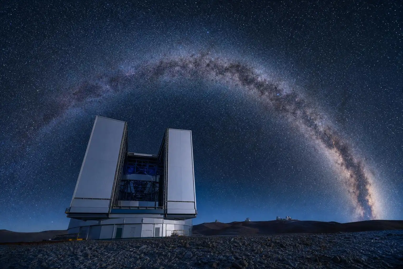

There is a moment, the first time you look at a MUSE data cube, when the sheer density of information becomes almost philosophical. You are staring at a three-dimensional array — two spatial axes, one wavelength axis — that contains a complete optical spectrum at every pixel across a patch of sky roughly one arcminute on a side. Point at a galaxy cluster. Point at a nearby dwarf galaxy. Point at the remnant of a supernova. Wherever you aim, MUSE hands you back not a photograph and not a single spectrum but something that is both at once, and more: roughly 90,000 spectra, each covering 480 to 930 nm, each with a spectral resolution of R ≈ 3,000, all gathered simultaneously in a single one-hour integration. Understanding why that is hard — and how the instrument actually does it — is the whole story.
The Problem Integral Field Spectroscopy Solves
Classical long-slit spectroscopy is a compromise. You orient a narrow slit across your target, disperse the light with a grating, and record a spectrum for each spatial position along the slit. One observation, one slice. If you want to map a galaxy’s velocity field, you must rotate the slit and repeat, or accept that you are only sampling one line through a complex, two-dimensional structure. The result is a patchwork of observations taken under different conditions, stitched together with uncertain systematics.
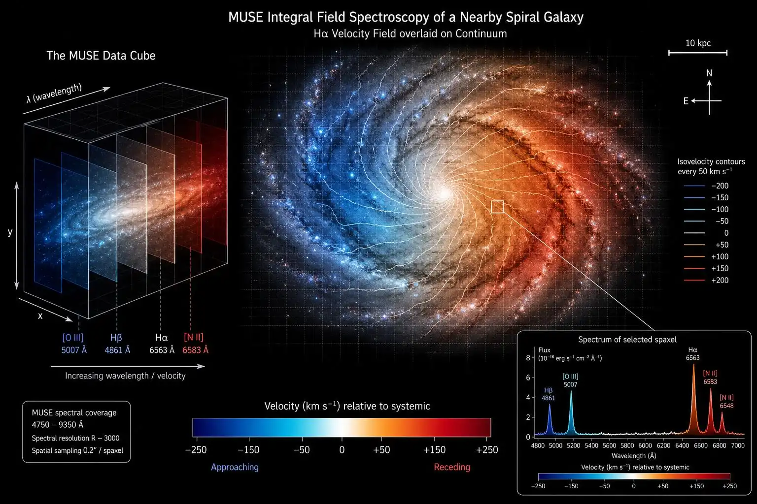
Integral field spectroscopy (IFS) breaks that compromise. Instead of a slit, you place an array of sampling elements — lenslets, fibers, or image slicers — at the focal plane. Each element captures light from a distinct spatial position. All of those beams are then reformatted, dispersed, and recorded simultaneously on a detector. You get spatial coverage and spectral coverage in one shot, with no temporal gaps between slices. The data product is a cube: two spatial dimensions and one spectral dimension, every voxel filled with a measured flux.
MUSE, the Multi Unit Spectroscopic Explorer, is the most ambitious realization of this idea ever built for an optical telescope. It sits at the Nasmyth focus of UT4 (Yepun) at the VLT on Cerro Paranal, Chile, and it achieves its scale through a design choice that is elegant and slightly terrifying: it uses not one integral field unit but twenty-four, working in parallel.
Twenty-Four Spectrographs, Twenty-Four Detector Systems
The heart of MUSE is its image slicer architecture. Light from the telescope arrives at the instrument’s entrance focal plane and is divided by a field splitter into 24 equal, adjacent rectangular sub-fields. Each sub-field is fed to its own dedicated integral field unit (IFU), which contains its own image slicer, its own collimator, its own diffraction grating, and its own 4k × 4k CCD detector. Twenty-four complete spectrographs, operating in parallel, each handling 1/24th of the field.
Within each IFU, the image slicer takes its rectangular sub-field and cuts it into 48 thin slices — narrow strips of sky, each about 0.2 arcseconds wide in the standard wide-field mode. These slices are then rearranged end-to-end into a pseudo-slit: a long, thin strip of reformatted sky. That pseudo-slit is dispersed by the grating, and the resulting spectrum of all 48 slices lands on the CCD. The detector records wavelength in one direction and the spatial position along the pseudo-slit (which encodes both the slice number and the position within that slice) in the other.
The full wide-field mosaic of all 24 IFUs together produces a 300 × 300 spaxel grid across the field. The field itself is sampled at 0.2 arcseconds per pixel in wide-field mode, covering 60 × 60 arcseconds total. The wavelength axis runs from 480 to 930 nm, sampled at 0.125 nm per channel, yielding 3,681 wavelength planes. The final data cube is 300 × 300 × 3,681 voxels — roughly 90,000 spectra, as advertised.
The Detector: Twenty-Four CCDs, One Coherent Dataset
Each of the 24 CCDs in MUSE is an e2v Technologies 4096 × 4096 chip with 15-micron pixels, operated at −130 °C to suppress dark current. The read noise is approximately 3 electrons per pixel per read, and the detectors are read out in about 40 seconds after an exposure. In a one-hour science integration, that read noise contribution is negligible compared to sky background photon noise — MUSE is sky-noise limited across the optical range, including at the reddest wavelengths where OH airglow makes the sky particularly bright, and is read-noise limited only in very short exposures.
Getting 24 independent CCDs to behave as a single coherent instrument is a calibration challenge of the first order. Each detector has its own bias structure, its own flat-field response, its own fringing pattern at red wavelengths (fringing arises from thin-film interference in the silicon as wavelength approaches the detector’s sensitivity cutoff near 930 nm). Each grating has its own wavelength solution, which must be tied to a common reference frame. Each image slicer introduces its own geometric distortion, which must be mapped with arc-lamp exposures and then corrected in the data reduction pipeline.
The MUSE pipeline — developed at the Institut für Astrophysik Göttingen and maintained by the consortium — processes all 24 channels simultaneously and merges them into a single data cube with a common spatial and wavelength grid. The resampling step, where 24 slightly different spatial samplings are interpolated onto one grid, is where you can lose signal-to-noise if you are not careful. The pipeline uses a drizzle-like algorithm to preserve flux while suppressing aliasing. In practice, the final cube is photometrically accurate to a few percent, which is sufficient for emission-line flux ratios, stellar velocity dispersions, and continuum colors across the field.
Wide-Field Mode, Narrow-Field Mode, and the Role of Adaptive Optics
MUSE operates in two primary modes. Wide-field mode (WFM) covers 60 × 60 arcseconds at 0.2 arcseconds per spatial pixel. In its standard seeing-limited configuration, spatial resolution is set by the seeing — typically 0.6 to 0.8 arcseconds at Paranal in the optical — and the instrument’s strength is sheer étendue: the product of collecting area and solid angle on sky. You are trading resolution for coverage, and for extended objects like galaxy clusters or nearby galaxies, that trade is almost always worth making.
Narrow-field mode (NFM) covers only 7.5 × 7.5 arcseconds at 0.025 arcseconds per pixel, but it is coupled to the VLT’s Adaptive Optics Facility (AOF) — specifically to the GALACSI module, which uses four laser guide stars and one natural guide star to correct atmospheric turbulence across the field. In NFM with AO, MUSE achieves a Strehl ratio of roughly 5 to 15 percent in the V band (around 550 nm), which sounds modest but translates to a point-spread function with a sharp diffraction core sitting on a broad seeing halo. At V band, the diffraction limit of an 8.2-meter telescope is about 14 milliarcseconds; MUSE NFM does not reach that limit, but it does deliver spatial resolution of 50 to 80 milliarcseconds — a factor of ten improvement over natural seeing.
The laser guide stars in the AOF are four sodium-layer beacons, each created by a 22-watt laser tuned to the sodium D2 line at 589.0 nm. The lasers excite sodium atoms in the mesosphere at 90 km altitude, creating artificial stars whose wavefront distortion is measured by Shack-Hartmann sensors and corrected by the deformable secondary mirror of UT4 — a 1.12-meter shell with 1,170 actuators, replacing the conventional secondary with a mirror that itself bends thousands of times per second. The natural guide star corrects the tip-tilt mode, which the laser guide stars cannot measure (because the laser beam traverses the atmosphere twice, the upward and downward paths cancel the global image motion). The result is a corrected wavefront delivered to MUSE NFM, enabling the kind of spatially resolved spectroscopy of dense stellar systems — globular clusters, galactic nuclei — that was previously impossible at optical wavelengths from the ground.
What You Do with 90,000 Spectra
The scientific payoff of a MUSE data cube is easiest to appreciate by example. Consider a single one-hour observation of a galaxy cluster at redshift z ≈ 0.5. In that cube, you will find:
Emission-line galaxies identified by their [O II] 3727 Å doublet, redshifted into the MUSE bandpass. A single cube can yield redshifts for hundreds of cluster members and background galaxies simultaneously, without any pre-selection. The Hubble Frontier Fields program used MUSE to confirm redshifts for lensed background galaxies as faint as magnitude 27, objects that would require multi-hour integrations with a traditional spectrograph — and even then, you would need to know in advance which objects to target.
Diffuse emission from the intracluster medium, from stripped gas tails behind infalling galaxies, from Lyman-alpha nebulae around high-redshift quasars. Because MUSE records every spatial position simultaneously, you do not need to know where the diffuse emission is before you observe. It simply appears in the cube, and you find it in post-processing by collapsing the wavelength axis around the relevant line.
Stellar kinematics in nearby galaxies. Fit the absorption lines — Mg b at 518 nm, the calcium triplet at 850–866 nm — at each spatial pixel, and you recover a two-dimensional map of stellar velocity and velocity dispersion. From that map, you can derive the galaxy’s dynamical mass, identify kinematically distinct components (a fast-rotating disk embedded in a slow-rotating bulge, for instance), and measure the mass of a central black hole if the spatial resolution is sufficient.
Planetary nebulae as kinematic tracers. In nearby elliptical galaxies, MUSE can detect individual planetary nebulae — dying stars that emit strongly in [O III] 5007 Å — across the entire galaxy in a single pointing. Each PN gives you a radial velocity, and the ensemble traces the dark matter halo far beyond the stellar body.
The Calibration Burden and Why It Is Worth It
Running MUSE is not simple. Every night, before science observations begin, the instrument requires a suite of calibrations: bias frames to measure the zero-level of each detector, flat-field exposures with a continuum lamp to map pixel-to-pixel sensitivity variations, arc-lamp exposures (typically with neon, argon, and xenon lamps) to establish the wavelength solution for each of the 24 spectrographs, and twilight sky flats to calibrate the large-scale illumination pattern. The pipeline ingests all of these, processes them in sequence, and produces a master calibration set that is applied to the science data.
Sky subtraction deserves special mention. The sky background — airglow emission lines from OH radicals in the upper atmosphere, a forest of narrow lines especially redward of 700 nm — must be removed from every spatial pixel. MUSE’s wide field is both an asset and a liability here: the asset is that some fraction of the field is almost always blank sky, which you can use to model the sky spectrum. The liability is that the sky spectrum varies slightly across the field and in time, and the instrument’s 24-channel architecture means that the sky model must be consistent across all 24 detectors. The Zurich Atmosphere Purge (ZAP) algorithm, developed specifically for MUSE, uses principal component analysis to separate sky residuals from source signal after the initial pipeline reduction. In practice, sky subtraction is the limiting factor for faint, extended emission — not detector noise, not read noise, but the residuals left after subtracting a sky that itself is not perfectly stable.
A Machine That Changed What Questions You Could Ask
MUSE saw first light in January 2014. In its first decade of operation, it has been used to discover Lyman-alpha halos around essentially every high-redshift galaxy observed at sufficient depth, to map the ionization state of gas in star-forming regions across entire nearby galaxies, to detect the faint stellar streams of disrupted satellite galaxies around the Milky Way’s neighbors, and to measure black hole masses in the nuclei of nearby galaxies through stellar kinematics — measurements that complement infrared and astrometric approaches at other facilities by providing independent dynamical constraints.
What MUSE represents, at the engineering level, is a commitment to multiplexing as a philosophy. The instrument is large — it fills a volume roughly 2 meters on a side and weighs about 8 tonnes — and it is mechanically complex, with 24 detector systems, 24 detector controllers, and a data rate that produces about 600 megabytes per raw exposure. The data reduction pipeline runs for tens of minutes on a modern computing cluster to produce a single science cube. None of this is free. But the payoff is that every photon collected by the telescope is assigned not just a position on the sky but a wavelength, and the ensemble of all those assignments tells you something no single spectrum and no single image ever could.
There is a discipline in that — in building an instrument so complex that its calibration is itself a research problem, so data-rich that its outputs require new analysis algorithms, so ambitious that it took a consortium of seven European institutions and more than a decade of development to realize. The pretty picture at the end, the false-color map of a galaxy’s velocity field or the emission-line portrait of a supernova remnant, is the surface. Underneath it are 24 synchronized spectrographs, about 402 million detector pixels, and a pipeline that has to agree with itself to better than one percent. That agreement, when it holds, is the real achievement.



Leave a Reply